Functional Safety Suite 7.0
User’s Guide
7 Fault Trees
7.1 Introduction and Overview
Fault tree analysis is the most common method for hazard analysis. The algorithms provided by Functional Safety Suite allow calculations of all values necessary for safety analysis or reliability analysis. In particular, adequate algorithms for calculation of occurrence rates related to repairable systems are implemented, therefore fault trees can also be used for occurrence rate (PFH, failure rate, hazard rate) calculations in accordance to [EN 61508], [EN 50126], [EN 50129], [ISO 13849], [ISO 26262-5] or similar.
Probably the most cited book related to fault tree analysis is the “Fault Tree Handbook” [NUREG], published in 1981 by the US Nuclear Regulatory Commission following the Three Mile Island accident in 1979. In 2002 NASA published the “Fault tree handbook with aerospace applications” [NASA]. Even though this book refers to [NUREG], its focus is different and just its existence already shows, that the spectrum of problems is too large to be explained in one book.
The most remarkable difference is, that in [NASA] the class of technical processes to be analyzed is a mission characterized by
-
• a defined start and end time
-
• no components serviceable or repairable during system lifetime
-
• no (safety related) undetected faults assumed at t=0
-
• no possibility to enter a safe state in case of a failure
-
• a probability p that the mission fails (equivalent to the unreliability F(0,Tmission)
whereas in [NUREG] as well as in all machinery or transportation related standards such as [EN 61508], [ISO 13849], [EN 50126], [ISO 26262-5] the problems can be characterized by
-
• a continuous process without defined start and end time
-
• maintenance including inspections and tests in certain intervals
-
• optionally a defined safe state of the overall system ([EN 61508]: ‘equipment under control’, EUC) that can be taken up in case of a detected failure
-
• repair possible either during operation or after (save) shut-down of the equipment under control (EUC)
-
• either a mean probability
 that all safety systems and (active) safety barriers fail when required (equivalent to their unavailability) — in [EN 61508] called “probability of failure on demand” (PFD)
-
• or a mean occurrence rate
 of dangerous system failures — in [EN 61508] called “probability of failure per hour” (PFH).
Both [NUREG] and [NASA] are available on the Internet for free and describe in detail the method of fault tree analysis. In addition they provide detailed information of how to construct a fault tree correctly. Therefore this documentation focuses
on the specific characteristics and the usage of Functional Safety Suite. Note that [EN 61025] does not cover repairable systems and hence is of very limited use (in particular, it doesn’t cover calculation of a system failure rate ).
According to [NUREG] a
fault tree is a graphic representation of the various parallel and sequential combinations of faults, that will result in the occurrence of the predefined undesired event.
In Functional Safety Suite it is even more: From version 7.0 on, fault trees can be simulated by Monte-Carlo-Simulation as an alternative to the “classic” evaluation via prime implicants (minimal cut-sets). Monte-Carlo-simulation permits a much more detailed and thus more realistic modeling and evaluation. In particular, gates and basic events have a state that changes over time both randomly and according to predetermined rules:
-
• randomly occurring faults let basic events change their state,
-
• determined test intervals let basic events change their state,
-
• states of some gates may affect the detection of faults of lower level basic events,
-
• the behavior of gates may depend on the sequence of input failures etc.
See section 7.4 for the available gate types. Using these new gate types, fault trees are better be described as
fault tree is a graphic representation of the various faults of components (or occurrence of other unwanted events), their detection, their technical and operational effects and reactions, and their parallel and sequential combinations that will result in the occurrence of the predefined undesired event.
Typically a fault tree analysis is used on a high level. A fault tree analysis is a deductive method, thus fault trees are always developed top-down (already having basic events in mind when starting to create a tree is one of the most common mistakes).
A basic event of a fault tree can describe the status of an element of the system (a situation or condition lasting for a while) or the occurrence of something in just a moment (a failure, or an action of the operator for instance).
Each basic event is assigned a failure or occurrence model with a specific set of parameters. Based on these parameters, the (conditional) occurrence rate h (unit 1/h), the unconditional
occurrence rate for repairable elements w (unit 1/h), the (unconditional) failure density F (unit 1/h), the unavailability Q, and the unreliability F can be calculated for each basic event. The occurrence rates h or w and the unavailabilities Q of the basic events are needed to calculate both occurrence rates and unavailabilities of higher level gates. The mean unavailability of the top event is the PFD, its mean occurrence rate is the PFH. For many systems, the system unreliability Fsys(0,Tmission), i. e. the probability of mission failure can directly be calculated
based on the unreliabilities F of the basic events. If there are conditions in the fault tree, i. e. elements that are described by their
unavailability Q instead of F, the system unreliability must be calculated based on the mean occurrence rate  or by the time-dependent failure density
  .
.
If used for THR apportionment (often named preliminary FTA), the values for the basic events are defined based on what seems realistic and achievable with reasonable effort. Thus, experience is necessary to perform a preliminary FTA. The parameters assigned to each basic event serve as the tolerable probability of failure on demand (TPFD) or tolerable failure rate (TPFH, TFFR), that has to be achieved by the responsible system element.
Features of Functional Safety Suite related to fault trees:
-
• correct calculation of occurrence rates also for repairable systems,
-
• many occurrence/failure models for basic events, including links to other fault trees, reliability block diagrams, Markov models and complex component,
-
• gates of many types, including several types suitable for Monte-Carlo simulation only (non-boolean gates, sometimes called “dynamic gates”),
-
• Combination gates with an arbitrary number of different inputs,
-
• Determination of the minimal cut-sets or prime implicants, even for huge trees,
-
• modularization using special TRANSFER-IN gates,
-
• the β-model for common cause factors,
-
• conversion of architecture diagrams to fault trees,
-
• conversion of fault trees to (extended) reliability block diagrams,
-
• conversion of fault trees to (extended) Markov models,
-
• check of fault trees according to [SiRF] rules,
-
• steady state evaluation,
-
• transient (time-dependent) evaluation,
-
• evaluation by Monte-Carlo-simulation.
Note: The structure of a fault tree is often more important with respect to the correctness of the derived conclusions than the actual quantitative values. It is absolutely necessary that the structure of a fault tree reflects reality and that no important events are omitted because of rules or “political” reasons. All relevant conditions (e. g. responsibilities, maintenance cycles etc.) must be known in order to enable the safety engineer to develop a correct fault tree. Where the relevant conditions are not known, assumptions can be used, but these must be mentioned explicitly. In fact for most systems a small number of critical elements (basic event) can clearly be determined, e. g. by a importance analysis (see section 11.6.2). It makes sense to concentrate on elements with high impact and to validate that they are correctly modeled.
7.2 The Fault Tree Properties
Presentation related properties of the fault tree are edited in the fault tree properties panel directly, see below. Evaluation related properties are set in the fault tree evaluation properties dialog, see section 7.6. All properties of the fault tree are stored in the fault tree file (extension .ftl).
7.2.1 General Properties
Description: A user defined description of the fault tree.
7.2.2 Presentation Properties
Note that in case the presentation related features don’t fulfil your needs, you can export all graphics in SVG format for further processing by vector graphics tools.
Horizontal offset: The margin between the window border and the left edge of the leftmost basic event. Standard is 5 [pixel] (multiplied by the zoom-factor). A bigger value makes sense for trees with few basic events in order to create space for the tree description (avoid overlap of description and top event).
Vertical offset: The margin between the window border and the upper edge of the top event. Standard is 5 [pixel] (multiplied by the zoom-factor).
Event width: Select the width of the name boxes in fault trees. The description boxes of basic events have the same width, description boxes of gates are about 20% wider.
Standard is 118 pixel, allowing to display both occurrence rate and unavailability in one line. If you only want to display unavailabilities or no values at all, you can enter a smaller width. If you need more space especially in description boxes, you can enter a larger width.
Header X Position: The margin between the window border and the left side of the header. Standard is 5 [pixel] (multiplied by the zoom-factor). You can shift the header to the right by setting to a higher value.
Show values: If values shall not be shown, you can switch them off here.
7.3 Tree Basic Events
A basic event of a fault tree consists of the reference to the generic basic event, an optional suffix, the ‘second text line’ (for qualitative fault trees only), and the background color.
The parameters in the ‘Tree Basic Event’ section belong to the specific basic event, which is part of a fault tree, and thus are stored in the fault tree file (extension .ftl).
The parameters in the ‘Generic Basic Event’ section belong to the generic basic event as selected by the field ‘GBE name’, and thus are stored in the library.
Remember: Changing parameters in the ‘Generic Basic Event’ section will change the properties of all other basic events referring to the same generic basic event too.
7.3.1 Tree Basic Event – General Properties
7.3.1.1 Package Select whether the generic basic event is in the library of the global package or of the local package.
7.3.1.2 GBE Name The identifier of the generic basic event, also serving as the name of the basic event. You can select a name (and by this the referred generic basic event) out of a list of the generic basic events belonging to the selected package.
Two possibilities exist with respect to common causes in general (also see section 7.7.1):
-
1. The same event is needed at multiple positions in the tree(s) (e. g. the system-wide loss of the main power supply): In this case either none or all of these events are true at a given time t. In EN 61025 this is called ‘repeated events’ or ‘replicated events’, within Functional Safety Suite it is called ‘identical events’. To tell the evaluation algorithm that you mean the same event everywhere, you must provide the same generic basic event and the same suffix to all of these events (or an empty suffix for all of them).
-
2. Multiple components of the same type are used in the system in a similar way (for instance in a 1oo2 or 2oo3-(sub)system). In that case these components will typically share some common cause failures. Their contribution can be set in the properties of the selected basic event. To tell the evaluation algorithm that it shall consider the given common cause factor between these components, you must use the same generic basic event (the same name) for all of them, but with different suffixes (e. g. ‘1’, ‘2’ and ‘3’ or ‘FRONT’ and ‘REAR’).
Thus the suffix is used to distinguish multiple basic events referring to the same generic basic event, that are not identical, but share a common cause factor β>0.
Since dots ‘.’ are used automatically to delimit the name from the suffix and also to indicate multiple parts of the suffix in prime implicants (cut-sets), they should not be used in the name or suffix (even it would be technically possible).
7.3.2 Tree Basic Event – Qualitative Properties
For qualitative fault trees a ‘second text line’ is displayed instead of the numeric values in the name field of each event. It doesn’t get lost when changing the project type in the project properties dialog to quantitative evaluation. Since this text is specific to each basic event, it is a property of the basic event, not the underlying generic basic event. Therefore it is stored in the fault tree file.
If you want to check the fault tree according to [SiRF]-rules, the ‘second text line’ must begin with either ‘SAS’ or ‘SL’, followed by one optional space, followed by a number 0 to 4. After that arbitrary text is allowed. Also see section 7.8 and the example provided with Functional Safety Suite.
7.3.3 Tree Basic Event – Background Color
The background color can be selected separately for each event.
7.3.4 Generic Basic Event – General Properties
A user defined description of the generic basic event and therefore identical for all basic events referring to this generic basic event.
7.3.4.2 House event, Condition event, Not developed
See section 4.2.1.
7.3.5 Generic Basic Event – Model
The probabilistic model of the generic basic event. See section 4.3 for details.
7.3.6 Generic Basic Event – Values
The values needed by the model of the generic basic event. See section 4.3 for details.
7.4 Gates
For mathematical evaluation based on prime implicants (minimal cut-sets) the following gate types are supported:
-
• OR
-
• AND
-
• COMBINATION (M-out-of-N)
-
• NOT
-
• INHIBIT
-
• IF-THEN-ELSE
-
• REDUCED-COMBINATION
-
• TRANSFER-IN
For Monte-Carlo-Simulation the gate types indicated in table 4 are available in addition. If a fault tree containing those gates is evaluated based on prime implicants instead of Monte-Carlo-Simulation, they are replaced by either the first input or by another gate type as indicated in column Replacement. The result will typically be conservative, but in some cases it might be optimistic (e. g. if basic events with decreasing failure rates are used and in case of a VOTING-AND).
| Type | Restrictions | Replacement |
| DIAGNOSIS | not in condition | first input only |
| DIAGNOSIS-INHIBIT | not in condition | AND |
| DIAGNOSIS-AND | AND | |
| VOTING-AND | COMBINATION | |
| PRIORITY-AND | AND | |
| REPLACEMENT | not in replacement | first input only |
| DIAGNOSIS-AND-REPLACEMENT | not in condition or replacement | first input only |
| SEQUENTIAL | not in spare or sequential | AND |
| SPARE | not in spare or sequential | input only |
| RESTORATION-ON-SAFE-FAILURE | first input only |
Some of these “gates” cannot be used in condition or replacement branches, see column Restrictions in table 4. Some of these “gates” influence the basic events in their branches. In that case, you might need to specify which basic events shall be affected by adding those basic events to a list, see the detailed description of each gate below and section 7.5.
Actually, only OR, AND, COMBINATION, NOT and IF-THEN-ELSE represent boolean combinations. The TRANSFER-IN-gate is just a structuring element not modeling any behavior of the system, see section 7.4.18 and section 7.7.2.1. All other “gates” are more semantic elements which make it possible to describe the behavior of this branch in the particular system precisely, considering operational aspects in a particular application, such as diagnosis, replacement and exact type of redundancy. These “gates” should be understood as tools to model the behavior in case of faults in the real application accurately. They will provide less conservative results compared to using boolean gates only and prevent using boolean gates in a wrong, non-conservative manner (such as misusing an AND-gate for diagnosis). In case of generic systems (element/system out of context), the assumptions leading to the usage of a specific gate type should be documented and exported as safety related application condition (SRAC).
Events connected to a gate are called ‘inputs’. The gate an event serves as input is called ‘parent’. The topmost event of a fault tree is called top event, in case of the highest level fault tree also ‘top hazard’.
If only one input is connected to a gate of type AND, DIAGNOSIS-AND, VOTING-AND or OR, the symbol is not displayed, since the gate has no effect.
Each input can be a basic event or another gate.
Common cause contributions are considered when calculating a gate, see section 7.7.1.
7.4.1 OR
-
• An OR-gate fails whenever one input fails (in Monte-Carlo-Simulation: only if no other input is failed already),
-
• is unavailable whenever any input is failed.

7.4.2 AND
-
• An AND-gate fails when all inputs are failed,
-
• is unavailable while all inputs are unavailable (i. e. until at least one is restored).

7.4.3 COMBINATION (M-out-of-N)
-
• A COMBINATION-gate fails if at least m inputs fail,
-
• is unavailable as long as at least m inputs are unavailable.

In fact the COMBINATION-gate is just an abbreviation of OR-ed AND-gates according to m and the number of inputs. Therefore calculation is done as with standard OR and AND-gates. You can check that by calculating and exporting the prime implicants or by exporting the resulting fault tree by Export – Final Fault Tree. Identical events or common cause factors between basic events contained in the branches below the COMBINATION gate will be considered as if it would be one single fault tree.
7.4.4 NOT
-
• A NOT-gate has one input,
-
• is unavailable while the input is ok (false),
-
• in Monte-Carlo-Simulation: a failure is counted when the input becomes false (ok), i.e. the occurrence rate is the same as the input occurrence rate, but the failure is set when the input is restored (transition from failed to ok).

Since the complement is defined for probabilities only, but not for rates or densities, a NOT-gate cannot deliver an occurrence rate to a higher level gate. Therefore it only makes sense in the condition branch of e. g. INHIBIT-gates or the diagnosis branch of e. g. DIAGNOSIS-gates, or if the unreliability F(t) shall be calculated.
7.4.5 INHIBIT
-
• An INHIBIT-gate has one input A and one condition input Cond,
-
• fails if the condition is true (failed) when the input A fails,
-
• is unavailable if it has failed until the input A is restored, (even if the condition Cond is not fulfilled any more already before).
-
• if the condition changes its state while the input A it still failed, the output does not change any more (i. e. if condition becomes true after the input A failed), the output will stay false (OK), and if the condition is not fulfilled any more (false, OK) while the input A is still failed, the output will stay failed until the input is restored.

Thus the INHIBIT-gate is similar to an AND-gate, except that the occurrence rate of the second input is ignored. Since the input A often describes a standard situation but not a failure, it is often a basic event marked as House Event.
Since the condition is quantified by a probability only (no occurrence rate), the basic events of the branch connected to the condition input should be marked with the modifier Condition Event, see section 4.2.1.1.
There are two special cases related to the condition input of an INHIBIT-gate:
-
1. If a generic basic event of type immediate is connected to the condition input and the parameter probability is set to zero, the branch topped by the INHIBIT-gate is completely ignored.
-
2. If a generic basic event of type immediate is connected to the condition input and the parameter probability is set to one, the condition input is ignored.
These rules might be useful in order to adapt the structure of a (generic) fault tree to different specific applications, i. e. to simplify the re-use of a fault tree for different projects. You can check the effect if you export the final fault tree by Export – Final Fault Tree.
When converting a fault tree to a Markov model, an INHIBIT-Gate will lead to instantaneous transitions.
An INHIBIT-gate is not allowed in the condition branch of a higher level gate.
Use Case An INHIBIT-gate is appropriate
-
• when the failure of the input A only matters if a (typically external) condition is (fulfilled)
-
• to reduce the effective failure rate and the unavailability by the probability of the condition being true (failed)
7.4.6 IF-THEN-ELSE (MUX)
-
• An IF-THEN-ELSE-gate has two inputs A and B and one condition input Cond,
-
• if the condition is true (failed) input A is considered for occurrence rate and unavailability,
-
• if the condition is false (OK) input B is considered for occurrence rate and unavailability,
-
• the condition is only considered at the time the input fails (i. e. a later change of the condition has no effect)
-
• only the input selected by the condition is considered, i. e. a change of the other input has no effect (even it is the one that has led to the failure of this gate before).

The gate’s occurrence rate and unavailability are input A times the probability Q of Cond, plus those of input B times the complementary probability 1–Q of Cond.
Note that due to the intended purpose of the gate, the two inputs A and B are mutually exclusive per definition, i. e. the combination of the two inputs is not included in the list of prime implicants.
Note that the use of this gate will form a non-coherent fault tree, including all the inconveniences non-coherent fault trees bring along (such as non-unique prime implicants or non-conservativeness even all failure rates are conservative).
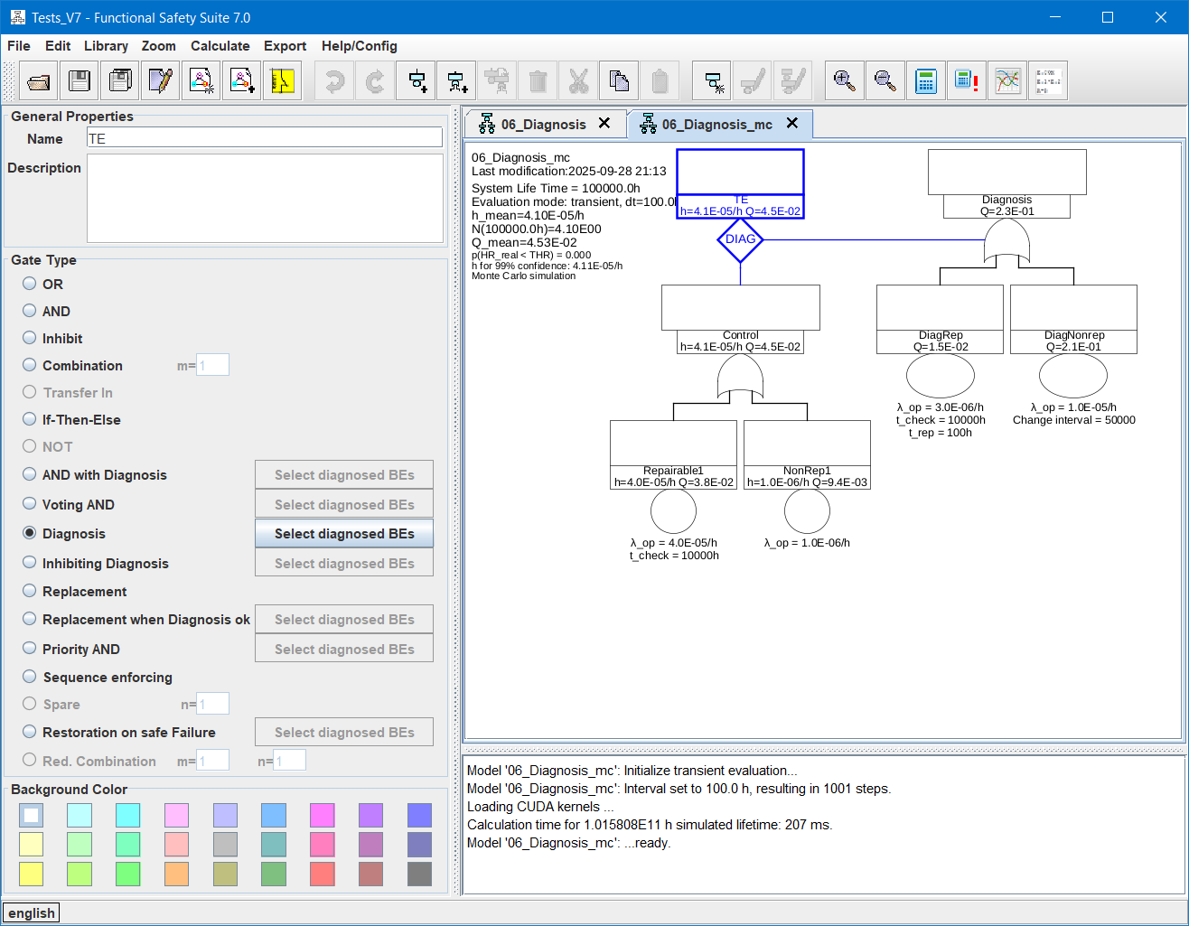
7.4.7 DIAGNOSIS
-
• A DIAGNOSIS-gate has one input A and one diagnosis input Diag,
-
• fails when the input A fails,
-
• is unavailable as long as the input A is failed (detected or undetected),
-
• if the input A fails while the diagnosis input is OK (false), some basic events will immediately set to repair state (or OK if trep=0), see below.

The failures of the following basic events will detected and the basic event sent to repair state (or to OK state directly if trep=0):
-
• if the input A is a basic event of type repairable or non-repairable, it will go to repair state, i. e. after trep it will be in OK state again,
-
• if the input A is a gate the user has to select the generic basic events whose failure will be detected out of a list containing all generic basic events of type repairable or non-repairable in branch A, see section 7.5.
-
• if the diagnosis is failed (diagnosis input true), the gate has no effect, i. e. the failures below input A will remain undetected until end of lifetime (for non-repairable) or until detected by the next periodic test (for repairable).
-
• independent and immediate diagnosis when input A fails
-
• reduce unavailability due to sleeping faults
-
• diagnostic coverage may be less than 100%, i. e. not all basic events below input A can be detected
Note: This gate has no effect on failure frequency, i. e. the gate will fail with the same frequency as the input A. Only the unavailability of input A will be reduced due to the detection. If the failure of input A is not dangerous at all if if is detected, the DIAGNOSIS-INHIBIT-gate might be the model of choice, see next section.
7.4.8 DIAGNOSIS INHIBIT
-
• A DIAGNOSIS-INHIBIT-gate has one input A and one diagnosis input Diag,
-
• fails if the diagnosis is failed when the input A fails (as for INHIBIT gate),
-
• is unavailable if it has failed until the input A is restored (as for INHIBIT gate),
-
• if the input A fails while the diagnosis input is false (OK), some basic events will immediately set to repair state (as for DIAGNOSIS gate, see there).

-
• independent immediate (=within PFTT) diagnosis when input A fails
-
• reduce unavailability due to sleeping faults
-
• only if the failure of the input A is safe if diagnosis is OK, i. e. system is forced to a safe state if detection is OK
Note: All failures of branch A must be detectable by the diagnosis if the diagnosis part is OK (false)! Failures not detectable by the diagnosis must be modeled in a parallel branch, connected by an OR-gate above this gate.
7.4.9 DIAGNOSIS-AND (AND with cross-wise diagnosis)
-
• A DIAGNOSIS-AND gate has an arbitrary number of inputs A, B etc.,
-
• fails if all inputs fail at the same time (either by the same basic event or by different basic events sharing a common cause) or when the last remaining input fails while the other inputs are still unavailable (i. e. the failure cannot be detected by another channel or still being repaired),
-
• is unavailable while all inputs are failed (i. e. until at least one is repaired),
-
• some basic events will immediately set to repair state if at least one input is OK (see below).

If at least one input is OK (false), any failures of the following basic events below failed inputs will detected and the basic event sent to repair state (or to OK state directly if trep=0):
-
• if a failed input is a basic event of type repairable or non-repairable, it will go to repair state, i. e. after trep it will be in OK state again,
-
• if a failed input is a gate the user has to select the generic basic events whose failure will be detected out of a list containing all generic basic events of type repairable or non-repairable in all branches, see section 7.5. Note: even no specific basic events but only generic basic events are selected for detection in the list, only failed basic events below a failed input of the DIAGNOSIS-AND gate will be detected, not below any (non-failed) input of the DIAGNOSIS-AND gate or somewhere else in the overall fault tree.
-
• multiple channels with cross-wise immediate (=within PFTT) diagnosis (with a
 )
)
-
• reduce unavailability due to sleeping faults
7.4.10 VOTING AND
-
• A VOTING-AND gate has an arbitrary number of inputs,
-
• fails if at least 50% of the available inputs fail at the same time,
-
• is unavailable after failure until more than 50% inputs are available again,
-
• some basic events might immediately be set to repair state if at least one input is OK (as for DIAGNOSIS-AND gate, see there).

Use Case This gate can be used if
-
• the majority of channels decide what is correct in case of discrepancy between channels,
-
• there is no safe state of the system (fail active operational design),
-
• there is no specific diagnosis in each channel, i. e. “diagnosis” is only comparison of the results and assumption that majority of outputs will be correct,
-
• optional: each channel can raise a failure information in some way in order to start the restoration.
7.4.11 REPLACEMENT
-
• A REPLACEMENT-gate has one input A and one replacement input R,
-
• the basic events of type standby repairable in the replacement input R are activated when input A fails,
-
• the basic events of type standby repairable in the replacement input R are deactivated when input A is OK again,
-
• the gate fails (gets true), if the replacement R fails at activation or while the input A is still failed,
-
• the gate is unavailable after failure until input A changes to OK (false).

-
• for component(s) in cold standby, that can fail at activation or during operation
-
• no diagnosis/complex activation to be modeled (e. g. detection of failure of A is guaranteed)
7.4.12 DIAGNOSIS REPLACEMENT
-
• A DIAGNOSIS-REPLACEMENT-gate is a combination of DIAGNOSIS / DIAGNOSIS-INHIBIT and REPLACEMENT,
-
• has one input A, one replacement input R and one diagnosis input Diag,
-
• fails if the diagnosis or the replacement R is failed when input A fails,
-
• fails if the replacement R fails at activation or while input A is still unavailable,
-
• is unavailable if it has failed until input A is restored,
-
• the basic events of type standby repairable in the replacement input R are activated when input A fails,
-
• the basic events of type standby repairable in the replacement input R are deactivated when input A is OK again,
-
• if input A fails while diagnosis is OK, some basic events of input A are immediately set to repair state (or OK if trep=0).

Use Case This gate describes a system with
-
• component(s) in cold standby, that can fail at activation or during operation,
-
• where the component(s) in cold standby are only activated if the diagnosis is working,
-
• with complex diagnosis containing many components that can fail as well or depend on further conditions.
7.4.13 PRIORITY AND
-
• A PRIORITY-AND-gate fails if the first input A failed before the second input B, the second before the third input C etc. until all inputs have failed (and not been restored before failure of the last input),
-
• is unavailable as long as no input is restored,
-
• if one input is OK (false) – no matter whether it has never failed yet or has been restored –, some basic events of all failed inputs on the right of this input are immediately set to repair state (or OK if trep=0), see below.

Example: Assume input A failed first, then input B. After that input A has been restored (due to some periodic test and restoration or exchange). Now that input A is OK while input B is failed, the failure of input B will be detected as for a DIAGNOSIS-AND gate:
-
• if the input B is a basic event of type repairable or non-repairable, it will go to repair state, i. e. after trep it will be in OK state again,
-
• if the input B is a gate the user has to select the generic basic events whose failure will be detected out of a list containing all generic basic events of type repairable or non-repairable in any branch (A, B and C), see section 7.5. Note: even no specific basic events but only generic basic events are selected for detection in the list, only failed basic events below a failed input of the PRIORITY-AND gate will be detected, not below any (non-failed) inputs of the PRIORITY-AND gate or somewhere else in the overall fault tree.
-
• If the top failure only occurs if the inputs fail in a specific sequence.
7.4.14 SEQUENTIAL
-
• A SEQUENTIAL-gate has one active input at any time,
-
• in the beginning the first input A is considered only, it is the active input,
-
• when the active input fails, the next input is activated and considered from now on,
-
• when the last (the rightmost) input fails, the gate fails,
-
• basic events of type non-repairable will be activated at t=0,
-
• basic events of type non-repairable spare and standby repairable will be activated when the particular input becomes the active one (i. e. cannot fail before the input is the active one).

-
• If there are alternative (typically degraded) operating modes in case the main component (main mode) fails.
-
• Similar to SPARE, but with different spare components.
-
• Typically the unreliability F is to be quantified for these kind of systems/applications.
7.4.15 SPARE
-
• A SPARE-gate has one input A, which indicates m elements of the same type,
-
• fails if its input failed more than m-spare times,
-
– Note: m=1 means, there is one spare, i. e. the gate fails when the input fails for the 2nd time,
-
-
• remains failed after it fails until end of lifetime,
-
• basic events of type non-repairable will be activated at t=0,
-
• basic events of type non-repairable spare and standby repairable will be (re-)activated after each failure.

-
• If there is only a limited number of spare parts available during the mission.
-
• Similar to SEQUENTIAL, but with identical spare components.
-
• Typically the unreliability F is to be quantified for these kind of systems/applications.
7.4.16 RESTORATION ON SAFE FAILURE
-
• A RESTORATION-ON-SAFE-FAILURE-gate has two inputs: input D contains the dangerous failures, input S contains the safe failures S,
-
• fails when input D fails,
-
• is unavailable as long as the input D is failed,
-
• certain basic events are restored when the safe input S fails.

When the safe input S fails, any failures of the following basic events below failed inputs will detected and the basic event sent to OK state (trep=0 assumed):
-
• if the input (D or S) is a basic event of type repairable or non-repairable, it will go to OK state,
-
• if the input (D or S) is a gate the user has to select the generic basic events whose failure will be restored out of a list containing all generic basic events of type repairable or non-repairable in both input branches, see section 7.5.
Use Case Most components or modules include many failure modes. Many of them directly lead to a safe state of the EUC, and need to be repaired before the EUC can be operated at all, therefore. Those failure modes (and only those!) are called ‘safe’ failures. The repair is often a replacement of a bigger module or assembly, thus undetected dangerous (‘dormant’) faults will be eliminated as well, even they haven’t been detected at all. Other dangerous (‘dormant’) faults might be detected (and corrected) in a mandatory commissioning test after repair. In effect, safe failures often lead to (known or unknown) elimination of dangerous faults in particular for components, that typically failing safely before or more often than failing dangerously. This effect can be modeled with a RESTORATION-ON-SAFE-FAILURE gate.
Note: In contrary to dangerous basic events, the rates of safe failures should be intentionally selected too low in order to get a conservative overall model.
7.4.17 REDUCED COMBINATION
-
• A REDUCED-COMBINATION-gate has one graphically displayed input, which symbolizes n elements of the same type,
-
• no common cause failure considered between the n elements,
-
• number of elements n is limited to 170.

The output of a REDUCED-COMBINATION gate is true (faulty), if at least m out of the n inputs are true (faulty).
In contrary to all other gates, REDUCED-COMBINATION gates numerically evaluate the input event (they calculate the unavailability Qin and occurrence rate hin or unreliability Fin of the connected input before evaluation of the fault tree containing the REDUCED-COMBINATION gate). Unavailability Qg and occurrence rate hg or unreliability Fg of the gate are then calculated as function of n, m, Qin and occurrence rate hin or unreliability Fin and stored in a new temporary generic basic event, referred by a new temporary (internal) basic event of type Link. The formulas used to calculate higher gates only consider this basic event and thus do not get information of the structure below the REDUCED COMBINATION gate.
The suffix of the temporary (internal) basic event can be set to ‘#’ in order to create multiple instances of the element described by the REDUCED COMBINATION gate in higher level fault trees. This is achieved by adding an ‘#’ at the end of the name of the REDUCED COMBINATION gate, also see section 7.7.1.
-
• When there is a large number of similar items, that fail independent of each other.
7.4.18 TRANSFER-IN
A TRANSFER-IN gate is a reference to another event defined by the name of the referred fault tree and the name of an event in the referred fault tree. The referred fault tree must either be a member of the same package or of the global package. The referred event can be any basic event or gate in the tree, not only the top event. The referred fault tree cannot be the tree the TRANSFER-IN gate belongs to. Regarding calculations, sub-trees referred by TRANSFER-IN gates are treated as if they would be stated directly in the higher level tree. Therefore you can split trees wherever you want.

Please note the possibilities for handling of basic event names and common cause factors as described in section 7.7.1.
Note: Circular references are forbidden for obvious reasons. They are detected in the evaluation, the evaluation will be aborted and the error indicated in the status bar.
You can open the referred fault tree by double-clicking the gate.
7.5 The Gate Event Properties Panel
All properties of the gate are stored in the fault tree file (extension .ftl).
7.5.1 General Properties
A user defined identifier of the gate. Every gate should have another identifier although this is not required by Functional Safety Suite.
A user defined description of the gate. The description of TRANSFER-IN gates is copied from the referred event, whenever you change the fields for the referred tree name or the referred event name.
7.5.2 Gate Type
For a description of each particular type see section 7.4 above. Depending on the type of the gate you might have to define which failure modes (i. e. which generic basic events) can be detected or restored. If you click the Select diagnosed BEs button, a dialogue will open showing all generic basic events of types repairable and non-repairable below the relevant inputs of the particular gate and a checkbox for each of them.
7.5.3 Qualitative Properties
For qualitative fault trees a ‘second text line’ is displayed instead of the numeric values in the name field. It is stored in parallel to the numeric values and therefore doesn’t get lost when changing the evaluation mode in the project properties dialog (tab Fault Trees & RBDs) and vice versa.
If you want to check the fault tree according to [SiRF]-rules, the ‘second text line’ must begin with either ‘SAS’ or ‘SL’, followed by one optional space, followed by a number 0 to 4. After that arbitrary text is allowed. Also see the example in the doc-directory.
7.5.4 Background Color
The background color can be selected separately for each gate.
7.6 Evaluation of Fault Trees
In case of quantitative evaluation the value of interest for each safety function is either
-
1. the mean unavailability on demand
(PFD),
-
2. the mean occurrence rate
(PFH),
-
3. or the probability of failure F(T) after system lifetime (or mission time) T.
A fault tree can be evaluated in a qualitative way as well, see section 7.6.3.1 and 7.8.
The value of interest and several parameters related to quantitative evaluation of fault trees are set in the fault tree evaluation properties dialog, see section 7.6.3 below.
To evaluate a fault tree, select Calculate – Calculate Model Values. First the final tree is determined, this is the fault tree in which all TRANSFER-IN gates have been replaced by the adequate branch and all REDUCED-COMBINATION gates have been replaced by a link to another model. Also INHIBIT gates might have been eliminated, see section 7.4.5. Circular references are detected and indicated in the message window before the evaluation starts. In case of conventional evaluation (no Monte-Carlo-simulation), some gates will be replaced in the final tree according to table 4 above. The final tree can be exported to a new fault tree by Export – Final Fault Tree, e. g. in order to check if all modules referred by TRANSFER-IN gates have been considered as intended, see section 11.7.9.
Results of the evaluation are displayed in the header of the fault tree. In case of quantitative evaluation, results are displayed in each event’s symbol as well, see section 7.6.3.1.
The quantitative evaluation is performed either based on prime implicants (identical to minimal cut-sets in case of coherent fault trees), or it is performed by Monte-Carlo simulation. Since the algorithms are completely different, they are described in different sections 7.6.1 and 7.6.2.
If a value of a generic basic event, the suffix of a basic event or the structure or evaluation parameters of the fault tree is changed, all values that might be affected by this change are automatically marked invalid and not displayed anymore, so that no inconsistent values are displayed.
7.6.1 Evaluation via Prime Implicants or BDDs
For evaluation via prime implicants and/or BDDs some gates will be replaced in the final tree according to table 4 above. After creating the final tree, prime implicants and/or binary decision diagrams (BDDs) describing the unavailability Q, the unreliability F and/or the occurrence rates h or densities w are created. Then all lower level models connected by links and all generic basic events are evaluated, so that finally the prime implicants and/or BDDs can be quantified. Depending on your choice in the Gate Calculation Mode panel, either only the top event is calculated or all gates.
7.6.1.1 Quantitative Steady-state Evaluation
A steady-state analysis is appropriate for all systems that are supposed to operate for many years, with certain test intervals and optionally some down-times for maintenance and repairs. Several parts of the system might be replaced or repaired
during the system’s lifetime. In case that all failures are detected in adequate time (either by continuous diagnosis, by periodic tests or by malfunction of the system), both the failure rate h (PFH) and the
unavailability Q (PFD) of the system don’t depend on its actual age, but will reach some pseudo-stationary state where both values will oscillate around a mean value. The frequency of this oscillation is equal to the
longest detection interval or a multiple of it. This is even correct in case the failure rates of some particular components depend on their specific age, if the lifetimes of these components are shorter than the system life time. The value of interest for
each safety function performed by such a system is either the mean unavailability on demand (PFD), or the mean occurrence rate (PFH). The related standard is mainly [EN 61508] and the derived standards. Examples for those systems are machines, cars, trains, air-crafts, chemical plants, power plants, etc. and their control systems.
A steady-state analysis is very fast, because all values have to be calculated only once (compared to transient analysis, where all values have to be calculated many times, see below).
Unfortunately, there is one major issue related to steady-state calculation of unavailabilities: The mean value of the product of two (or more) time-variant values is in general not equal to the product of the mean values but greater:

The unavailability function Q(t) of a repairable component is a periodic function: It becomes Q(t)=0 after each (complete) test at time  and increases until the next test at time
  .
.
The following examples show the unavailability as function of time for a system of two repairable (and therefore periodically tested) components. The first example considers non-redundant components (connected by an OR gate), the second considers redundant components (connected by an AND gate).
A safety system consists of two components (both needed, not redundant) with two failure events E1 and E2.
E1 has a failure rate of  and is tested every 150 h.
E2 has a failure rate of  and is tested every 30 h.
Figure 35 shows the unavailability function Q(t) if at t0=0 both components are tested. Due to the given test intervals, also at  both components will be tested in parallel. The dotted lines are the single event unavailabilities, the solid line shows the overall unavailability, which is approximately the sum of both single event unavailabilities.
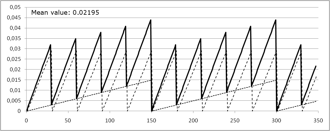
Figure 36 shows the unavailability function Q(t) if the test for E1 is executed at t1=t0, whereas the test for E2 is executed at t2=t0+15 h. Since there is no complete test, the overall unavailability never evaluates to 0 (at least not for t>0).
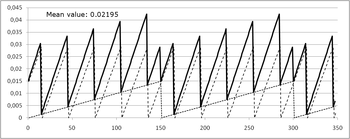
Note that the mean value is the same, independent of the relation of the test times.
The lifetime is usually much longer than a period of Q(t), because the component is tested or maintained several times during the lifetime.
Another special case is that the component/function is used only for one mission, e. g. it is created/tested before or at the start of the mission and becomes invalid after the end of the mission. In that case the interval is identical to the mission time.
A safety system consists of two redundant subsystems S1 and S2. S1 has a failure rate of and is tested every 150 h. S2 has a failure rate of and is tested every 50 h. With these values the mean unavailability of S1 is  , of S2 it is
  . Multiplication of both values gives
  .
.
Figure 37 shows the unavailability function Q(t) if at t=0 h both subsystems are tested.
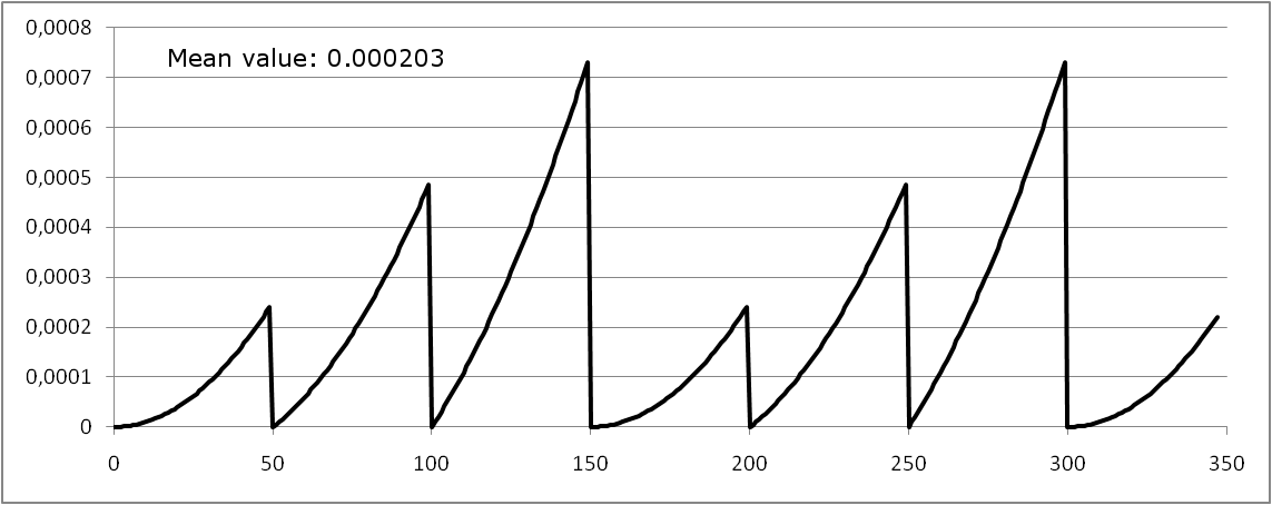
The mean unavailability is  but not ! Simple multiplication of the values is obviously not correct and not even conservative.
Figure 38 shows the unavailability function Q(t) if the test for S1 is executed at t1=0 h, whereas the test for S2 is executed at t2=15 h.
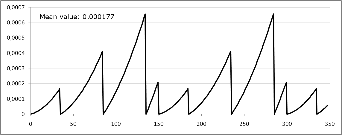
With this shift the mean unavailability is  , with a shift of t2=25 h it would be
  .
.
As shown in example 2, when performing the conjunction of events (using an AND-gate) the mean overall unavailability is not given by the product of the mean unavailabilities of each event. For synchronized tests without shift, the mean unreliability of the system is always higher than the product of the mean unavailabilities of its events. Also refer to [EN 61508-6], section B.2.2.
Thus, using mean values of the components unavailabilities is too optimistic in general. One option is to use maximum values of the components (basic events) unavailabilities, i. e. the unavailability just before the next test, but this is quite pessimistic. Functional Safety Suite provides three options on how to deal with this issue in steady-state evaluations, see section 7.6.3.4. The only way how to calculate the exact values is using a transient evaluation, but this needs much more computing time, unfortunately.
7.6.1.2 Quantitative transient Evaluation
A transient (or time-variant) analysis typically produces more precise results for
-
• fault trees or Markov models containing basic events with time-variant parameters, e. g. basic events of type non-repairable,
-
• fault trees or Markov models including basic events of type cyclic.
-
• fault trees resulting in minimal cut-sets that are longer than 2 events.
Also if the ‘mission failure probability’, namely the system’s unreliability F(0,Tmission) is the value of interest, a transient evaluation usually makes sense, even though many systems of this kind can also be modeled by steady-state fault trees or Markov models, using generic basic events of type non-repairable, see section 4.3.2.
The step size for transient evaluation in hours. A smaller step size means more steps for the given system lifetime and thus takes more time in calculation. This might be an issue in case of large systems. The step size must be less than a 10th of the smallest periodic (cyclic) event you want to evaluate for discrete times. Time constants less than 10 times the step size are handled as rates. However step size should be even smaller in order to reduce the computational errors.
7.6.2 Evaluation via Monte Carlo Simulation
In contrary to all other algorithms, the Monte-Carlo simulation is not implemented in Java code but in C++ and CUDA® and compiled to separate libraries in order to speed up simulation. It requires either a Nvidia® GPU or MS Windows.
Minimal cut-sets (or prime implicants in case of incoherent fault trees) only contain basic events but no gates, thus they can only describe boolean combinations of basic events. They cannot describe sequences of effects that depend on the order of events, nor can they distinguish effects to basic events that depend on the state of other events. Those effects can nevertheless be described using the fault tree notation by introducing non-boolean “gates”, see section 7.4. Quantification of those (extended) fault trees however requires a Monte-Carlo simulation. Since a Monte-Carlo simulation is no mathematical calculation but a simulation of a random experiment, the more random experiments are simulated the more precise and reliable the result will be. One experiment is the simulation of one system over its lifetime. The number of experiments to be performed depends on which tolerable unavailability Qtol, tolerable failure frequency htol or tolerable unreliability Ftol you want to prove, and how close to this tolerable value the actual value of your system is. Thus, it is not possible to define the necessary number of experiments prior to doing the simulation, but only to estimate the statistic confidence of the result.
See section 7.6.4 for explanation of the parameters.
In addition to the simulation result, two values are stated in the model header:
-
1. the confidence that the simulation result is in fact less than the tolerable value entered in the parameters (see paragraph 7.6.4)
-
2. the value that can be guaranteed with a confidence of 99%
For Monte Carlo simulation, there is basically no difference between steady-state and transient evaluation — the simulation is identical. The difference is, that in transient evaluation, it will be recorded when a failure or restoration occurs. This will slightly increase simulation time and is only beneficial if you want to analyze the results in a chart, see section 11.6.5. Note that you’ll need a huge number of simulations in order to get a somewhat smooth chart, many more than necessary to get the overall result.
7.6.3 Evaluation Parameters
Note: If the fault tree is referred in another fault tree by a TRANSFER-IN gate, these parameters are irrelevant, since this fault tree will just be a branch of the final tree of the higher fault tree during evaluation.
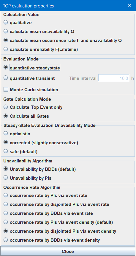
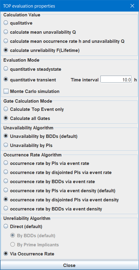
7.6.3.1 Calculation Value Select which value(s) to calculate:
-
• If qualitative is selected, the following operations are performed:
-
– determination of minimal cut-sets of a fault tree or reliability block diagram.
-
– optionally check a fault tree for consistency based on rules (version 7.0 includes an algorithm to check the rules stated in the [SiRF]).
Events of fault trees provide a second text line in the name field below the name, intended to be used to indicate some “safety level” or another qualitative specifier. The content of the second text line can be entered separately for each event and belongs to this event, not to the generic basic event (as the quantity related values do). This is necessary, because the “safety levels” of events (=component failures) of qualitative fault trees (maybe better called “occurrence rate levels” or “unavailability levels”) are often determined top-down (similar to a THR apportionment) and therefore different levels might be applied to the same (generic) event at different positions. The second text line is stored together with the gate or basic event in the fault tree file — even if the type is set to quantitative. See section 7.8 for more information.
-
-
• If calculate mean unavailability Q is selected, only
is calculated. In case of a transient evaluation, Q(t) is available for display in a chart frame.
-
• If calculate mean occurrence rate h and unavailability Q is selected, in addition to
and the estimated number of occurrences of the top event N(T) is calculated based on or h(t), see below. In case of a transient evaluation, also the unconditional failure density f(t), the semi-conditional failure rate w(t) and the
unreliability F(t) are calculated and available for display in a chart frame, in addition to h(t), Q(t), N(t).
-
• If calculate unreliability F(Lifetime) is selected, at least F(t) is calculated. If the unreliability is calculated directly, i. e. based on the unreliabilities of the basic events (see section 7.6.3.7), in case of the transient evaluation, also the unconditional failure density f(t) is calculated and thus can be displayed in a chart frame in addition to F(t). If the unreliability is calculated via occurrence rate, the same algorithms are used as if calculate mean occurrence rate h and unavailability Q would be selected, but instead of
and the unreliability F(t) is displayed in the graphics. Consequently, in case of a transient evaluation h(t), f(t), w(t), F(t), Q(t) and N(t) are available in the chart frame.
Depending on the selection, the parameters dialog will be adapted in order to show only the relevant parameters, see figure 39 and figure 40 for examples.
Select whether the fault tree shall be evaluated in steady-state mode or in transient (time-variant) mode.
Also select whether Monte Carlo simulation shall be used.
In case of transient evaluation, the time interval must be set as well. For transient evaluation based on prime implicants or BDDs, you can use a quite small step size, such as 10 h or even 1 h. For transient evaluation by Monte Carlo simulation, at most 10000 steps are allowed, but you should go for about 1000 steps.
Usually you should calculate all gates, because the intermediate gate values typically help understanding the fault tree and the critical paths. However, in order to save calculation time, you might want to calculate the top event only.
Calculate top event only: Only the top event of the fault tree is calculated, but no lower gates. This option just saves evaluation time, the top results will be the same.
Calculate all gates: All gates of the active fault tree are calculated. Select this option if you want to analyze where the top event’s results come from.
7.6.3.4 Steady-State Evaluation Unavailability Mode
Optimistic In ‘optimistic’ mode, the mean unavailabilities of generic basic events are used, as calculated according to section 4. As explained here before, this is usually optimistic.
Corrected In ‘corrected’ mode, also mean unavailabilities of generic basic events are used, but combinations of unavailabilities are multiplied by a factor greater than 1 (depending on the length of the cut-set), so that the result is for sure not too optimistic (however it might be pessimistic). Unfortunately this correction cannot be performed on BDDs directly, and thus if unavailability is calculated by BDDs (see section 7.6.3.5) the BDDs need to be converted to a sum of products of events, what requires quite some calculation effort for large fault trees.
Safe In ‘safe’ mode, the maximum unavailabilities of generic basic events are used, as calculated according to section 4. Obviously this is pessimistic for most basic event types, and the longer the cut-sets, the more pessimistic is the result.
Hint: If a fault tree contains components modeled by basic events of type repairable, standby or link, that are tested at the same time and only rarely (e. g. in a preventive maintenance once per month or year), so that their unavailabilities are not obviously negligible, you should perform a transient evaluation instead of a steady-state evaluation to get precise results. If a fault tree contains non-repairable events, you should always go for transient evaluation.
7.6.3.5 Unavailability Algorithm
Calculation by BDDs Calculations based on BDDs are both accurate and very fast even for huge fault trees. The only reason not to select this option is in steady-state evaluation with unavailability mode ‘corrected’ (see section 7.6.3.4) for big fault trees.
Calculation by PIs Calculations based on PIs are more or less pessimistic due to missing disjointedness between cut-sets (or prime implicants). The only reason to select this option is in steady-state evaluation with unavailability mode ‘corrected’ (see section 7.6.3.4) for big fault trees.
7.6.3.6 Occurrence Rate Algorithm
If the minimal cut-sets (or prime implicants, PIs) of a fault tree are known, the occurrence rate of the top event hsys can be estimated based on the occurrence rates and unavailabilities of the basic events by

The PIs are determined by an algorithm using modified BDDs (in fact ternary decision diagrams, TDDs), which is very fast. The evaluation of the PIs doesn’t need much memory, but some computing time. In case of high unavailabilities ( ) this estimation can be too conservative. However, since such high unavailabilities shouldn’t occur in a safety related system, the estimation is sufficiently precise for most problems.
In case of high unavailabilities, a more precise estimation can be calculated based on the (unconditional) occurrence density wsys and the unavailability Qsys:
![(35) \begin{equation} w_{\mathrm {sys}}=\sum _{i=1}^{n_{\mathrm {PI}}} \left ( \left [ \sum _{j=1}^{n_{\mathrm {Lit,PI_i}}} \left ( w_j \cdot \prod _{k=1,k\neq j}^{n_{\mathrm {Lit,PI_i}}} q_{i,k} \right )
\right ] \cdot \prod _{j=1,j\neq i}^{n_{\mathrm {PI_j}}} \left ( 1-\prod _{k=1}^{n_{\mathrm {Lit,PI_j}}} q_{j,k} \right ) \right ) \end{equation}](fusasu-images\image-138.svg)

This algorithm obviously needs some more calculations and is therefore slower.
Both algorithms are conservative estimations also due to the fact, that the prime implicants are not disjointed. The exact calculation requires disjointed prime implicants, which need to be determined by converting the PIs to BDDs again, one BDD per literal. This is a resource intense operation and thus is only possible for small to medium size fault trees. But once the BDDs have been created (if they can be created with given memory resources), numerical evaluation will be very fast.
In addition to these algorithms, an algorithm not using PIs at all is implemented, i. e. the occurrence rate is directly calculated by BDDs. This is the fasted algorithm. Unfortunately there is no formal proof of the correctness (or at least conservativeness), therefore you shouldn’t rely on it before having it crosschecked by another algorithm.
All possible combinations of algorithms are available for selection. Algorithms using the occurrence rates of the basic events are always somewhat faster than their counterparts using unconditional occurrence frequencies (by a factor of 2 approximately).
occurrence rate by PIs via rate The occurrence rate is calculated based on the occurrence rates and unavailabilities of the basic events contained in the PIs. Doesn’t need much memory, but high computing effort for transient evaluation. Result is conservative, in particular for high unavailabilities or large fault trees.
occurrence rate by disjointed PIs via rate PIs are sorted for literals and then being disjointed by BDDs. The occurrence rate is then calculated based on the occurrence rates and unavailabilities of the basic events. Needs much memory, but only medium computing effort for transient evaluation. Result is slightly conservative, in particular for high unavailabilities or large fault trees.
occurrence rate by BDDs via rate The occurrence rate is directly calculated based on BDDs, using occurrence rates and unavailabilities of the basic events. No PIs are determined. Needs few memory and only small computing effort for transient evaluation. Result might not be correct for some trees (deviates from PI based algorithms in both directions).
occurrence rate by PIs via density The occurrence rate is calculated based on the occurrence densities and unavailabilities of the basic events contained in the PIs. Doesn’t need much memory, but high computing effort for transient evaluation. Result is conservative, in particular for large fault trees.
occurrence rate by disjointed PIs via density PIs are sorted for literals and then being disjointed by BDDs. The occurrence rate is then calculated based on the occurrence densities and unavailabilities of the basic events. Needs much memory, but only medium computing effort for transient evaluation. Gives the correct result.
occurrence rate by BDDs via density The occurrence rate is directly calculated based on BDDs, using occurrence densities and unavailabilities of the basic events. No PIs are determined. Needs few memory and only small computing effort for transient evaluation.
7.6.3.7 Unreliability Algorithm
Up to version 4 of Functional Safety Suite, the unreliability has been calculated based on the occurrence rate or h(t). This method is suitable for all kinds of systems, but a little conservative and quite slow. Version 5 provides an algorithm to calculate the unreliability directly. This is quite simple and fast, and in fact this is how all “traditional”
fault tree tools calculate unreliability, and what is explained in all books including [EN 61025]. Unfortunately, this is wrong in case the fault tree contains conditions, as demonstrated in the following example.
Example 3:
A top event ‘TE’ occurs, whenever a periodic event ‘H’ appears and a condition ‘Cond’ is fulfilled when ‘H’ appears. This is modeled in the fault trees shown in figure 41. Event
h appears every 1000 hours with a probability of 0.1. Thus, given a system lifetime of 200 000 hours, it will appear about 20 times (of course this is no fix value, but the expected value). In
the left fault tree, the top event’s unreliability is calculated “directly”, i. e. by  . Even though both FH and QCond are probabilities, they must not be multiplied, because they are different quantities. The correct result has to be
calculated based on the occurrence rate by
. Even though both FH and QCond are probabilities, they must not be multiplied, because they are different quantities. The correct result has to be
calculated based on the occurrence rate by  with
with  , as shown on the right.


Thus if the fault tree doesn’t contain conditions, select Direct, if it contains conditions select Via Occurrence Rate.
In case of direct calculation of the unreliability, you can select whether it shall be calculated By BDDs or By Prime Implicants (minimal cut-sets). In fact there is no reason for using prime implicants — it is much slower than via BDDs and the result is pessimistic (by BDDs the result is exact).
If the unreliability F(t) is calculated via occurrence rate (), in steady-state evaluation it is calculated by

and in transient evaluation it is calculated by

For small values of N ( , as fulfilled typically for higher level events),
  is valid. For lower level events h often does not have the meaning of a failure rate, but determines usually occurring events, so that often
  applies for a longer system lifetime, and
  accordingly.
7.6.4 Evaluation Parameters – Monte-Carlo Simulation
When the Monte Carlo simulation checkbox is selected, the Monte Carlo Simulation Parameters panel (figure 42) is shown instead of the panels described above.
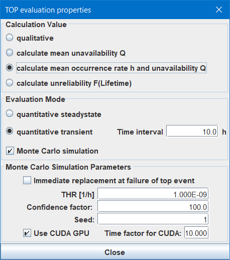
Set checkbox Immediate replacement at failure of top event if the system described by the fault tree is completely replaced when the top even occurs. This will lead to reset of all time variant generic basic events in the fault tree in case of the top failure. The effect will only be visible in case of a quite high top event failure rate.
7.6.4.2 Tolerable Unavailability, Tolerable Hazard Rate, Tolerable Unreliability
Depending on the selected calculation value (see section 7.6.3.1) the tolerable unavailability Qtol, the tolerable hazard rate THR or the tolerable unreliability Ftol can be entered. The smaller the tolerable value, the more simulations will be performed, see next paragraph.
In addition, this value is used for calculation of the achieved probabilistic confidence, see section 7.6.2.
Since it is not possible to calculate the necessary number of simulations for a given tolerable value or required confidence prior to the simulation, the number of simulations to be performed needs to be selected by the user. One simulation means the simulation of one instance of the system over its lifetime as defined in the project properties dialog.
The number of simulations nsim is calculated as follows, depending on the calculation value, the tolerable value, the system lifetime T and the confidence factor c:
- Q:
-

- h:
-

- F:
-

The Monte Carlo simulation uses pseudo random numbers during evaluation. With the same seed you’ll get the same result whenever you perform a calculation (given all other parameters are the same as well, of course). 6 If you for some reason want to perform a different random experiment, set another value here.
If your computer is equipped with a (not too old) Nvidia® GPU, you can use the CUDA libraries provided with Functional Safety Suite. This will typically speed up simulation by 20 to 1000 times — depending on the exact GPU.
The GPU driver will cancel the calculation after a few seconds. (leading to a restart of the GPU driver that might come along with some short flickering of your monitor). Functional Safety Suite tries to estimate the complexity of the simulation and will split the simulation of one system lifetime into shorter parts when necessary. In order to avoid those failures, you might need to adjust this value to smaller values. Larger values typically don’t make sense since only simple simulations might speed up a little bit, but they are quite fast anyhow.
7.7 Modularization and Common Causes
7.7.1 Handling of Common Causes
Two common cause scenarios are to be considered:
-
1. Multiple events in the fault tree(s) depict the identical event and have therefore the same name and suffix. If those events are conjuncted via AND or COMBINATION gates, all duplicates are deleted in the minimal cut-set, thus the common cause factor stated in the basic event properties is meaningless.
-
2. Multiple events in the fault tree(s) refer to different components in the system and therefore have the same name X (pointing to the same generic basic event X) but different suffix. In that case, when calculating the unavailability and occurrence rate of a minimal cut-set, the common cause factor β stated in the basic event properties is considered. Therefore the generic basic event X is split into two generic basic events internally: One containing the single-cause part
 and
and  , the other containing the common-cause part
  and
and  . The generic basic event of the common cause part has the same name X, but a suffix COM, as you can see in the minimal cut-set list (see section 11.6.3).
See figure 43 for an example. Given two components X.1 and X.2 of same type X. A common cause factor β of 1% is assumed between components of this type due to their construction, manufacturing and environment. For one function ‘A’ at least one of the two components X.1 and X.2 is needed, in another function ‘B’ component X.1 and another component Y is needed.
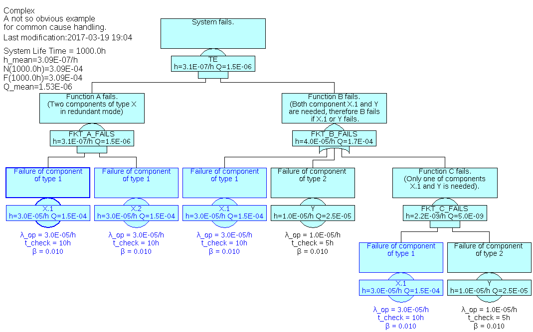
As expected, a common cause factor of 0.01 is used between the two components X.1 and X.2 of the same type X (see the values of ‘FKT_A_FAILS’) whereas events X.1 are treated as the identical event: ‘FKT_B_FAILS’ has no impact to the top event since event X.1 in ‘FKT_B_FAILS’ will always occur whenever event ‘FKT_A_FAILS’ occurs (obviously such a system architecture makes no sense). ‘FKT_B_FAILS’ is not even calculated, since component Y doesn’t occur in the cut-sets at all and therefore is not initialized. You can check the cut-sets by clicking Calculate – Show Minimal Cut-sets.
Note that if a basic event is selected, all basic events referring to the same generic basic event as the selected one are highlighted in blue color as well (see figure 43). This applies also to basic events in other models, thus when you switch to another model, you can also directly see the related basic events.
7.7.2 Modularization of Fault Trees
For the same reasons as in other fields of engineering, it usually makes sense to split a complex system into several ‘modules’ or ‘units’. This is the same for fault trees. In fact one will aim to reflect the architecture of the system in the fault trees.
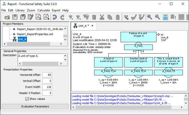
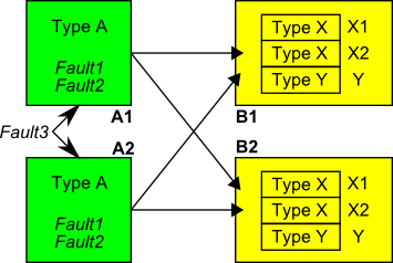
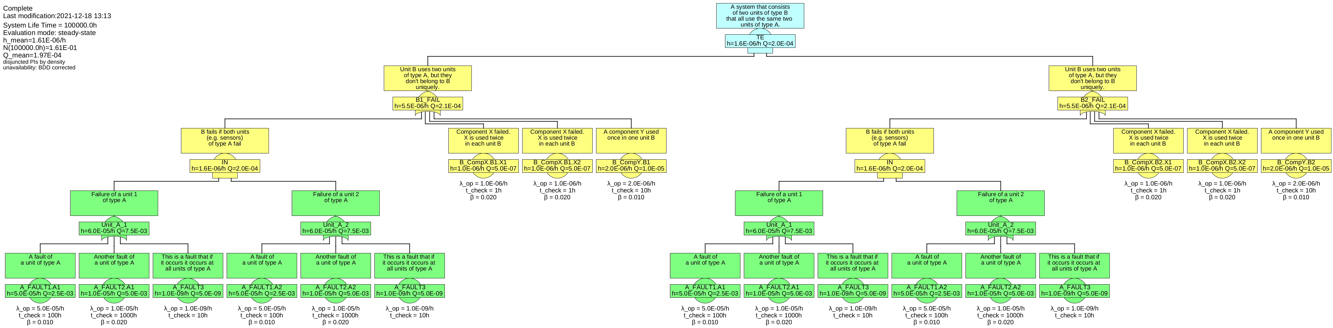
See figure 44 for an example of a system, consisting of four modules, characterized as follows:
-
• The overall system consists or two units of type B, named B1 and B2.
-
• The overall system fails, when both units B1 and B2 fail.
-
• Each unit of type B includes two components of the same type X, named X1 and X2 per unit B.
-
• Each unit of type B includes one component of type Y.
-
• Each unit of type B uses the same two external units of type A, named A1 and A2.
-
• A unit of type B fails, when both units A1 and A2 fail, or any of its own components X1, X2 or Y.
-
• Each unit of type A can fail due to three faults, FAULT1, FAULT2, FAULT3.
-
• FAULT3 will always let all units of type A fail.
Units A could be sensors, whereas B1 and B2 could be computers working with the sensor data.
The fault tree of this system is shown in figure 45.
At least if units A and B are even more complex, you’ll feel a need to split this tree into several sub-trees. In principle Functional Safety Suite provides two possibilities: TRANSFER-IN gates and links.
7.7.2.1 Modularization by TRANSFER-IN gates
Apart from dividing large fault trees to several pages, gates of type TRANSFER-IN are used in two cases:
-
1. the same unit is needed for multiple higher level units or (sub-)functions. In that case, the TRANSFER-IN gates referring to the sub-tree shall represent the same unit and thus the identical event.
-
2. a unit is existing twice or more in the system. In that case, the sub-tree describes one of these units. The fault tree uses multiple TRANSFER-IN gates referring to this sub-tree, whereas each TRANSFER-IN gate shall represent a different unit and thus different events.
The two cases are handled in a simple way in Functional Safety Suite:
-
• If the names of TRANSFER-IN gates are equal, the referred sub-trees are considered to relate to the same unit (case 1).
-
• If the names of TRANSFER-IN gates differ, the referred sub-trees are considered to relate to different units (case 2).
However imagine that in case 2, the sub-tree refers to some events, that are not specific to each unit described by this sub-tree, but shared by all units of this kind (and maybe even other units). In order to describe also this case correctly, the following rule applies:
Rule 1: If the suffix of a basic event ends with ‘#’, a new basic event will be created internally when constructing the cut-sets during calculation. The suffix of the new basic event will be the name of the TRANSFER-IN gate plus ‘.’ plus the original suffix (excluding the ‘#’). 7
In case of multiple levels of TRANSFER-IN gates, the names of all TRANSFER-IN gates will be stringed together, separated by ‘.’ and starting with the lowest level.
By this mechanism, the overall example system could now be split as shown in figures 46 and 47.

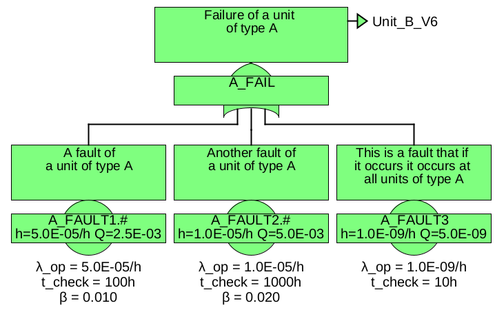
The suffixes ‘#’ of ‘A_Fault1’ and ‘A_Fault1’ will be extended to ‘A1’ and ‘A2’. Now you might also want to model units of type B with one generic fault tree B. If you’d just replace the gates ‘B1_Fail’ and ‘B2_Fail’ by TRANSFER-IN gates, rule 1 would apply again. Thus the suffixes ‘#’ of ‘A_Fault1’ and ‘A_Fault1’ would be extended to ‘A1.B1_Fail’, ‘A1.B2_Fail’, ‘A2.B1_Fail’ and ‘A2.B2_Fail’, i. e. you’d model independent units A1 and A2 for each of the units B1 and B2. But remember, that the same units (sub-tree) A1 and A2 are needed in all units of type B. So you’ll have to tell in tree B, that you mean identical A’s in all instances of B.
Therefore the following rule applies:
Rule 2: If the name of the TRANSFER-IN gate ends with ‘%’ 8, or if a
transfer extension is stated, the names of higher level TRANSFER-IN gate names will be ignored.
Given this, it is possible to split the top tree as shown in figure 48.

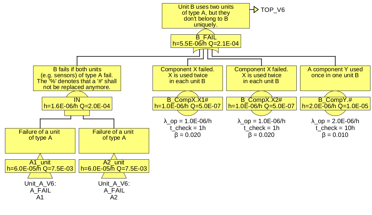
each referring to the same two generic units of type A.
In any case you can check the result by having a look at the list of minimal cut-sets (see section 11.6.3). It should always be as shown in table 5.
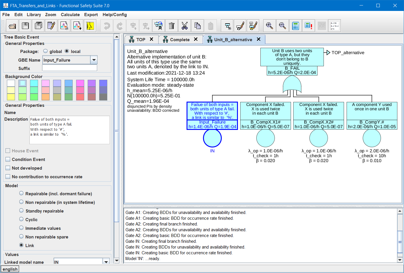
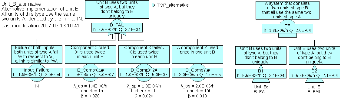
7.7.2.2 Modularization by Links
The linking mechanism (see sections 2.4 and 4.3.7) provides another possibility to split fault trees. In the given example, it can be used as shown in figure 49. The difference to using a TRANSFER-IN gate is, that the link hides all internal details of ‘IN’ from fault trees using this link.
7 Prior to version 6.0, the complete original suffix including the ‘#’ has been appended. From version 6.0 on, the ‘#’ is omitted in the final fault tree, because it’s not needed anymore.
8 Note: The name of the TRANSFER-IN gate must not be ‘%’ only.
7.7.3 REDUCED-COMBINATION Gates and deleting Common Cause Contributions
In contrary to all other gates, REDUCED-COMBINATION gates numerically evaluate the list of minimal cut-sets of the input event (they calculate qi and hi of the input). Unavailability qg and occurrence rate hg of the gate are then calculated as function of n, m, qi and hi and stored in a new temporary generic basic event, referred by a new temporary basic event. Minimal cut-sets of higher level events only contain this basic event and thus do not contain lower level information including any common cause factor.
Since they reduce information, they are called ‘Reduced’ Combination gates. This reduction has three reasons:
-
1. Implicit conversion to AND and OR gates as done in standard COMBINATION gates is not feasible any more for very large number of inputs (n).
-
2. The calculation of Q and h based on minimal cut-sets is not accurate if the same events occur in many cut-sets. The calculation error is typically
 and therefore negligible, but when the same events occur in hundreds or thousands of cut-sets, it is not negligible any more. Correct calculation by disjointing the cut-sets on the other hand is by far too expensive especially for those
cut-sets, where it would be necessary.
and therefore negligible, but when the same events occur in hundreds or thousands of cut-sets, it is not negligible any more. Correct calculation by disjointing the cut-sets on the other hand is by far too expensive especially for those
cut-sets, where it would be necessary.
-
3. For many problems, a common cause between similar components is not assumed any more on a certain higher level (e. g. common causes have to be considered for components of the same type in one box, but several boxes of this type don’t share all those common causes any more since they are located far away from each other). Therefore a mechanism is needed to cut these low-level common causes in higher levels — which is provided by this kind of gate.
The suffix of the temporary (internal) basic event can be set to ‘#’, in order to create multiple instances of the element described by the REDUCED-COMBINATION gate in higher level trees. This is achieved by adding an ‘#’ at the end of the name of the REDUCED-COMBINATION gate.
7.8 Specifics of qualitative Fault Trees
The decision, whether fault trees are qualitative or quantitative is defined in the Evaluation properties of each fault tree, see section 7.6.3. 9 No data gets lost if the type is changed between qualitative and quantitative (steady-state or transient). Thus it is possible to use the same
project and the same fault tree for qualitative and quantitative evaluation.
Events of qualitative fault trees are sometimes classified in some way. For example a ‘safety level’ (SL) is assigned to each of them. Therefore qualitative fault trees provide a second text line, displayed in the name field below the name, intended to be used to indicate some “safety level” or another qualitative specifier. The content of the second text line can be entered separately for each event and belongs to this event, not to the generic basic event (as the quantity related values do). This is intended due to the fact, that the “safety levels” of events of qualitative fault trees are often determined top-down and therefore different safety levels might be assigned to the same event in different trees — or even within different branches of the same tree.
The second text line is stored together with the gate or basic event in the fault tree file (.ftl).
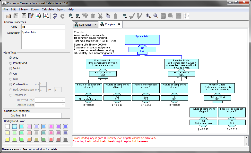
Since there is no mathematical rule how to “calculate” the SL of a gate based on the SL’s of the input gates or basic events, this task has to be performed manually. Therefore when evaluation type ‘qualitative’ is selected, the second line can be filled with an arbitrary text — as for example the assigned SL.
Nevertheless there might be rules of how to assign or apportion classes or SL’s. One example are the rules defined for the authorization of railway vehicles in Germany ([SiRF]). Functional Safety Suite includes an algorithm to check qualitative fault trees according to the [SiRF] rules.
The qualitative evaluation is always based on minimal cut-sets.
9 Up to version 6.0 it was a project parameter, from version 7.0 you can select for each fault tree separately.
7.9 Editing of Fault Trees
Create a fault tree by File – New Model. Select a name and package for the new tree that will be created. Finally a simple fault tree, only consisting of the top gate, is created.
Select the top gate by clicking on it. Add a gate below by Edit – Add Gate.
Add a basic event based on a new generic basic event below the selected gate by Library – New Generic Basic Event. After entering a name, a new generic basic event will be created, and a basic event referring to this generic basic event will be added below the selected gate. Note that the new generic basic event is created in the local package of the fault tree by default, but you can also choose to create it the global package.
Add a basic event referring to an existing generic basic event below the selected gate by Edit – Add Tree Basic Event. The new basic event will refer to the latest generic basic event by default. You can select any other existing generic basic event by selecting it via its name and package in the Tree Basic Event Properties Panel, see section 7.3.
The sequence of events below a gate can be changed by ‘Shift- ’ and ‘Shift-
 ’.
’.
A gate or a basic event can be deleted with the ‘Delete’ key. In case of a gate, the inputs of the deleted gate will be added to the parent gate.
A branch can be deleted by ‘Shift+Delete’.
If you want to assign a new (not yet existing) generic basic event to an existing basic event, select Library – New Generic Basic Event. The name of the basic event will change to the name of the new generic basic event, showing that it now refers to the new generic basic event.
You can copy or cut branches by selecting the top gate of the branch and pressing ‘Ctrl+C’ or ‘Ctrl-X’. The branch saved like this can be pasted below any gate of the same or another fault tree by ‘Ctrl+V’. Neither the names of the gates nor the suffixes of the basic events of the pasted branch will be changed automatically, so it’s up to you to change them according to their new meaning and relation to other events.
Changing properties of gates or basic events is done in the properties window. The only exception is the change of the name of a generic basic event, for which a special command Library – Rename Generic Basic Event is foreseen. The properties of the generic basic event referred by a basic event can be edited in the library view as well, see section 4.1.
A fault tree that has not been saved after the latest modification is marked with an asterisk ‘*’ in its title.